![[Deprecated]](figures/lifecycle-deprecated.svg)
gg_subseries(data, y = NULL, period = NULL, ...)Arguments
- data
A tidy time series object (tsibble)
- y
The variable to plot (a bare expression). If NULL, it will automatically selected from the data.
- period
The seasonal period to display. If NULL (default), the largest frequency in the data is used. If numeric, it represents the frequency times the interval between observations. If a string (e.g., "1y" for 1 year, "3m" for 3 months, "1d" for 1 day, "1h" for 1 hour, "1min" for 1 minute, "1s" for 1 second), it's converted to a Period class object from the lubridate package. Note that the data must have at least one observation per seasonal period, and the period cannot be smaller than the observation interval.
- ...
Additional arguments passed to geom_line()
Value
A ggplot object showing a seasonal subseries plot of a time series.
Details
gg_subseries() was soft deprecated in feasts 0.4.2. Please use ggtime::gg_subseries() instead.
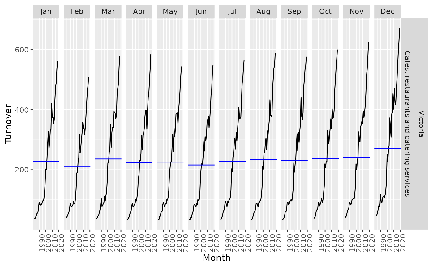
A seasonal subseries plot facets the time series by each season in the seasonal period. These facets form smaller time series plots consisting of data only from that season. If you had several years of monthly data, the resulting plot would show a separate time series plot for each month. The first subseries plot would consist of only data from January. This case is given as an example below.
The horizontal lines are used to represent the mean of each facet, allowing easy identification of seasonal differences between seasons. This plot is particularly useful in identifying changes in the seasonal pattern over time.
similar to a seasonal plot (gg_season()), and
References
Hyndman and Athanasopoulos (2019) Forecasting: principles and practice, 3rd edition, OTexts: Melbourne, Australia. https://OTexts.com/fpp3/