The function ACF computes an estimate of the autocorrelation function
of a (possibly multivariate) tsibble. Function PACF computes an estimate
of the partial autocorrelation function of a (possibly multivariate) tsibble.
Function CCF computes the cross-correlation or cross-covariance of two columns
from a tsibble.
ACF(
  .data,
  y,
  ...,
  lag_max = NULL,
  type = c("correlation", "covariance", "partial"),
  na.action = na.contiguous,
  demean = TRUE,
  tapered = FALSE
)

PACF(.data, y, ..., lag_max = NULL, na.action = na.contiguous, tapered = FALSE)

CCF(
  .data,
  y,
  x,
  ...,
  lag_max = NULL,
  type = c("correlation", "covariance"),
  na.action = na.contiguous
)
Arguments
- .data
A tsibble
- ...
The column(s) from the tsibble used to compute the ACF, PACF or CCF.
- lag_max
maximum lag at which to calculate the acf. Default is 10*log10(N/m) where N is the number of observations and m the number of series. Will be automatically limited to one less than the number of observations in the series.
- type
character string giving the type of ACF to be computed. Allowed values are
"correlation"(the default),"covariance"or"partial".- na.action
function to be called to handle missing values.
na.passcan be used.- demean
logical. Should the covariances be about the sample means?
- tapered
Produces banded and tapered estimates of the (partial) autocorrelation.
- x, y
a univariate or multivariate (not
ccf) numeric time series object or a numeric vector or matrix, or an"acf"object.
Value
The ACF, PACF and CCF functions return objects
of class "tbl_cf", which is a tsibble containing the correlations computed.
Details
The functions improve the stats::acf(), stats::pacf() and
stats::ccf() functions. The main differences are that ACF does not plot
the exact correlation at lag 0 when type=="correlation" and
the horizontal axes show lags in time units rather than seasonal units.
The resulting tables from these functions can also be plotted using
autoplot() with the methods provided by the ggtime package.
References
Hyndman, R.J. (2015). Discussion of "High-dimensional autocovariance matrices and optimal linear prediction". Electronic Journal of Statistics, 9, 792-796.
McMurry, T. L., & Politis, D. N. (2010). Banded and tapered estimates for autocovariance matrices and the linear process bootstrap. Journal of Time Series Analysis, 31(6), 471-482.
See also
Examples
library(tsibble)
#>
#> Attaching package: ‘tsibble’
#> The following objects are masked from ‘package:base’:
#>
#> intersect, setdiff, union
library(tsibbledata)
library(dplyr)
#>
#> Attaching package: ‘dplyr’
#> The following objects are masked from ‘package:stats’:
#>
#> filter, lag
#> The following objects are masked from ‘package:base’:
#>
#> intersect, setdiff, setequal, union
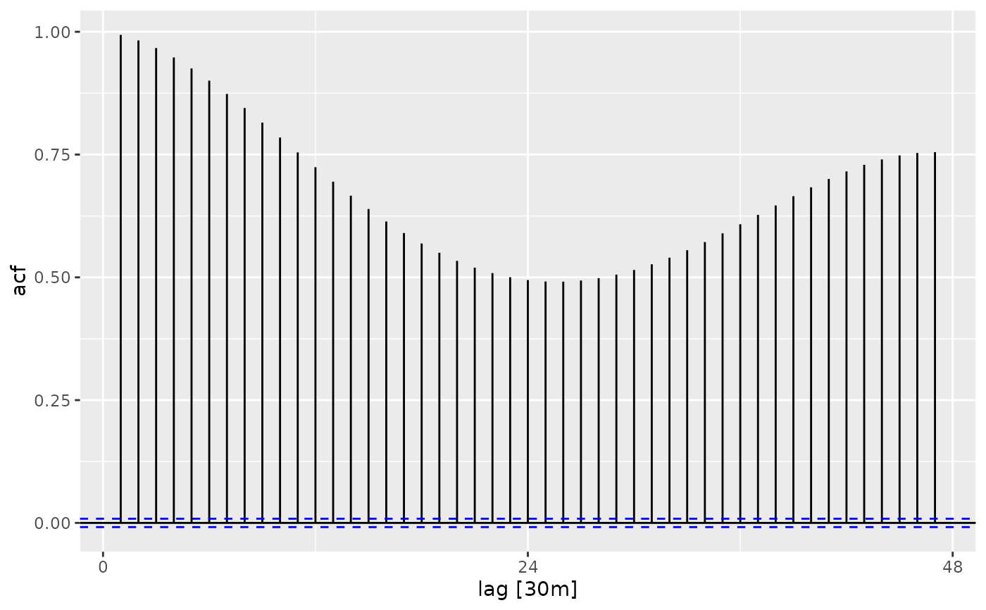
vic_elec %>% ACF(Temperature)
#> # A tsibble: 47 x 2 [30m]
#> lag acf
#> <cf_lag> <dbl>
#> 1 30m 0.994
#> 2 60m 0.982
#> 3 90m 0.967
#> 4 120m 0.948
#> 5 150m 0.925
#> 6 180m 0.901
#> 7 210m 0.873
#> 8 240m 0.845
#> 9 270m 0.815
#> 10 300m 0.785
#> # ℹ 37 more rows
vic_elec %>% ACF(Temperature) %>% autoplot()
#> Plot variable not specified, automatically selected `.vars = acf`
#> Don't know how to automatically pick scale for object of type
#> <cf_lag/vctrs_vctr>. Defaulting to continuous.
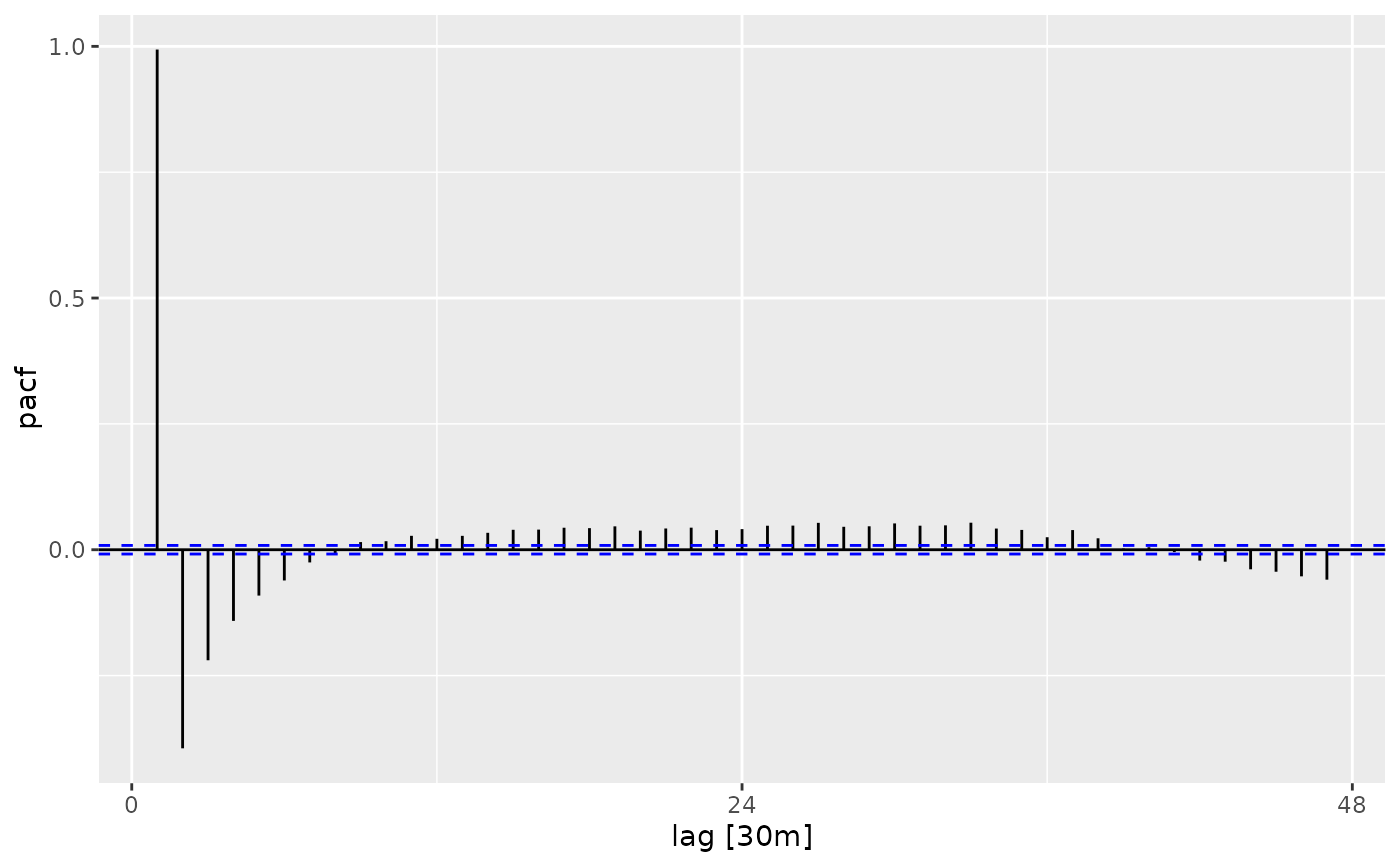
 vic_elec %>% PACF(Temperature)
#> # A tsibble: 47 x 2 [30m]
#> lag pacf
#> <cf_lag> <dbl>
#> 1 30m 0.994
#> 2 60m -0.395
#> 3 90m -0.220
#> 4 120m -0.141
#> 5 150m -0.0911
#> 6 180m -0.0611
#> 7 210m -0.0252
#> 8 240m -0.0101
#> 9 270m 0.0152
#> 10 300m 0.0169
#> # ℹ 37 more rows
vic_elec %>% PACF(Temperature) %>% autoplot()
#> Plot variable not specified, automatically selected `.vars = pacf`
#> Don't know how to automatically pick scale for object of type
#> <cf_lag/vctrs_vctr>. Defaulting to continuous.
vic_elec %>% PACF(Temperature)
#> # A tsibble: 47 x 2 [30m]
#> lag pacf
#> <cf_lag> <dbl>
#> 1 30m 0.994
#> 2 60m -0.395
#> 3 90m -0.220
#> 4 120m -0.141
#> 5 150m -0.0911
#> 6 180m -0.0611
#> 7 210m -0.0252
#> 8 240m -0.0101
#> 9 270m 0.0152
#> 10 300m 0.0169
#> # ℹ 37 more rows
vic_elec %>% PACF(Temperature) %>% autoplot()
#> Plot variable not specified, automatically selected `.vars = pacf`
#> Don't know how to automatically pick scale for object of type
#> <cf_lag/vctrs_vctr>. Defaulting to continuous.
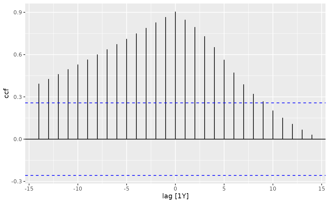
 global_economy %>%
filter(Country == "Australia") %>%
CCF(GDP, Population)
#> # A tsibble: 29 x 3 [1Y]
#> # Key: Country [1]
#> Country lag ccf
#> <fct> <cf_lag> <dbl>
#> 1 Australia -14Y 0.394
#> 2 Australia -13Y 0.427
#> 3 Australia -12Y 0.461
#> 4 Australia -11Y 0.496
#> 5 Australia -10Y 0.530
#> 6 Australia -9Y 0.565
#> 7 Australia -8Y 0.601
#> 8 Australia -7Y 0.637
#> 9 Australia -6Y 0.674
#> 10 Australia -5Y 0.711
#> # ℹ 19 more rows
global_economy %>%
filter(Country == "Australia") %>%
CCF(GDP, Population) %>%
autoplot()
#> Plot variable not specified, automatically selected `.vars = ccf`
#> Don't know how to automatically pick scale for object of type
#> <cf_lag/vctrs_vctr>. Defaulting to continuous.
global_economy %>%
filter(Country == "Australia") %>%
CCF(GDP, Population)
#> # A tsibble: 29 x 3 [1Y]
#> # Key: Country [1]
#> Country lag ccf
#> <fct> <cf_lag> <dbl>
#> 1 Australia -14Y 0.394
#> 2 Australia -13Y 0.427
#> 3 Australia -12Y 0.461
#> 4 Australia -11Y 0.496
#> 5 Australia -10Y 0.530
#> 6 Australia -9Y 0.565
#> 7 Australia -8Y 0.601
#> 8 Australia -7Y 0.637
#> 9 Australia -6Y 0.674
#> 10 Australia -5Y 0.711
#> # ℹ 19 more rows
global_economy %>%
filter(Country == "Australia") %>%
CCF(GDP, Population) %>%
autoplot()
#> Plot variable not specified, automatically selected `.vars = ccf`
#> Don't know how to automatically pick scale for object of type
#> <cf_lag/vctrs_vctr>. Defaulting to continuous.