Overview
feasts provides a collection of tools for the analysis of time series data. The package name is an acronym comprising of its key features: Feature Extraction And Statistics for Time Series.
The package works with tidy temporal data provided by the tsibble package to produce time series features, decompositions, statistical summaries and convenient visualisations. These features are useful in understanding the behaviour of time series data, and closely integrates with the tidy forecasting workflow used in the fable package.
Installation
You could install the stable version from CRAN:
install.packages("feasts")You can install the development version from GitHub with:
# install.packages("remotes")
remotes::install_github("tidyverts/feasts")
Usage
library(feasts)
library(tsibble)
library(tsibbledata)
library(dplyr)
library(ggplot2)
library(lubridate)
Graphics
Visualisation is often the first step in understanding the patterns in time series data. The package uses ggplot2 to produce customisable graphics to visualise time series patterns.
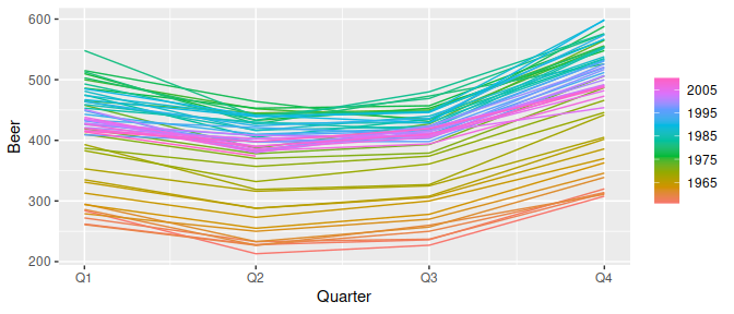
aus_production %>% gg_subseries(Beer)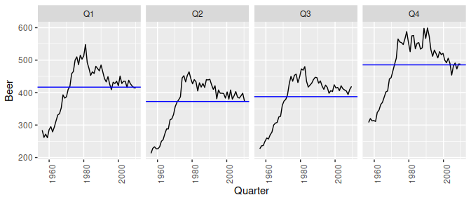
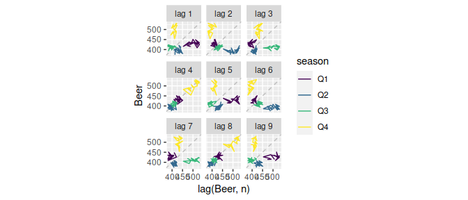
aus_production %>% ACF(Beer) %>% autoplot()
#> Plot variable not specified, automatically selected `.vars = acf`
#> Don't know how to automatically pick scale for object of type <cf_lag/vctrs_vctr>. Defaulting to
#> continuous.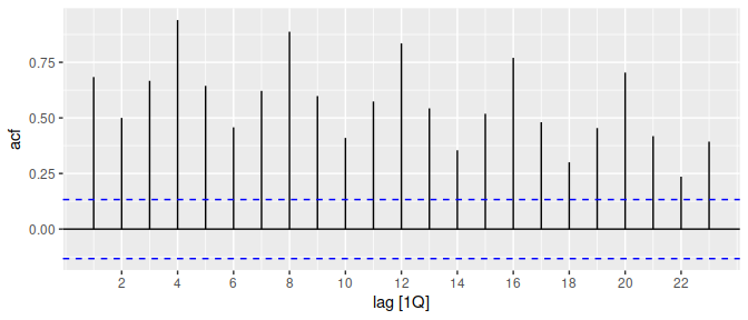
Decompositions
A common task in time series analysis is decomposing a time series into some simpler components. The feasts package supports two common time series decomposition methods:
- Classical decomposition
- STL decomposition
dcmp <- aus_production %>%
  model(STL(Beer ~ season(window = Inf)))
components(dcmp)
#> # A dable: 218 x 7 [1Q]
#> # Key:     .model [1]
#> # :        Beer = trend + season_year + remainder
#>    .model                           Quarter  Beer trend season_year remainder season_adjust
#>    <chr>                              <qtr> <dbl> <dbl>       <dbl>     <dbl>         <dbl>
#>  1 STL(Beer ~ season(window = Inf)) 1956 Q1   284  272.        2.14     10.1           282.
#>  2 STL(Beer ~ season(window = Inf)) 1956 Q2   213  264.      -42.6      -8.56          256.
#>  3 STL(Beer ~ season(window = Inf)) 1956 Q3   227  258.      -28.5      -2.34          255.
#>  4 STL(Beer ~ season(window = Inf)) 1956 Q4   308  253.       69.0     -14.4           239.
#>  5 STL(Beer ~ season(window = Inf)) 1957 Q1   262  257.        2.14      2.55          260.
#>  6 STL(Beer ~ season(window = Inf)) 1957 Q2   228  261.      -42.6       9.47          271.
#>  7 STL(Beer ~ season(window = Inf)) 1957 Q3   236  263.      -28.5       1.80          264.
#>  8 STL(Beer ~ season(window = Inf)) 1957 Q4   320  264.       69.0     -12.7           251.
#>  9 STL(Beer ~ season(window = Inf)) 1958 Q1   272  266.        2.14      4.32          270.
#> 10 STL(Beer ~ season(window = Inf)) 1958 Q2   233  266.      -42.6       9.72          276.
#> # ℹ 208 more rows
components(dcmp) %>% autoplot()
#> Warning: Using `size` aesthetic for lines was deprecated in ggplot2 3.4.0.
#> ℹ Please use `linewidth` instead.
#> ℹ The deprecated feature was likely used in the ggtime package.
#>   Please report the issue to the authors.
#> This warning is displayed once per session.
#> Call `lifecycle::last_lifecycle_warnings()` to see where this warning was generated.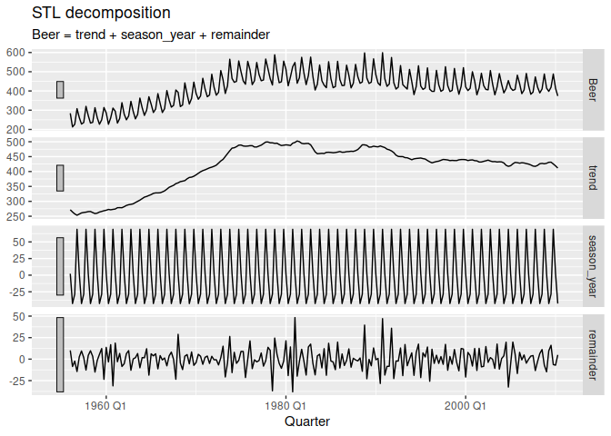
Feature extraction and statistics
Extract features and statistics across a large collection of time series to identify unusual/extreme time series, or find clusters of similar behaviour.
aus_retail %>%
  features(Turnover, feat_stl)
#> # A tibble: 152 × 11
#>    State      Industry trend_strength seasonal_strength_year seasonal_peak_year seasonal_trough_year
#>    <chr>      <chr>             <dbl>                  <dbl>              <dbl>                <dbl>
#>  1 Australia… Cafes, …          0.989                  0.562                  0                   10
#>  2 Australia… Cafes, …          0.993                  0.629                  0                   10
#>  3 Australia… Clothin…          0.991                  0.923                  9                   11
#>  4 Australia… Clothin…          0.993                  0.957                  9                   11
#>  5 Australia… Departm…          0.977                  0.980                  9                   11
#>  6 Australia… Electri…          0.992                  0.933                  9                   11
#>  7 Australia… Food re…          0.999                  0.890                  9                   11
#>  8 Australia… Footwea…          0.982                  0.944                  9                   11
#>  9 Australia… Furnitu…          0.981                  0.687                  9                    1
#> 10 Australia… Hardwar…          0.992                  0.900                  9                    4
#> # ℹ 142 more rows
#> # ℹ 5 more variables: spikiness <dbl>, linearity <dbl>, curvature <dbl>, stl_e_acf1 <dbl>,
#> #   stl_e_acf10 <dbl>
This allows you to visualise the behaviour of many time series (where the plotting methods above would show too much information).
aus_retail %>%
  features(Turnover, feat_stl) %>%
  ggplot(aes(x = trend_strength, y = seasonal_strength_year)) +
  geom_point() +
  facet_wrap(vars(State))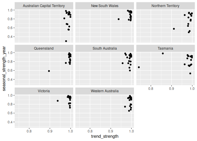
Most of Australian’s retail industries are highly trended and seasonal for all states.
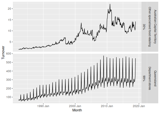
It’s also easy to extract the most (and least) seasonal time series.
extreme_seasonalities <- aus_retail %>%
  features(Turnover, feat_stl) %>%
  filter(seasonal_strength_year %in% range(seasonal_strength_year))
aus_retail %>%
  right_join(extreme_seasonalities, by = c("State", "Industry")) %>%
  ggplot(aes(x = Month, y = Turnover)) +
  geom_line() +
  facet_grid(vars(State, Industry, scales::percent(seasonal_strength_year)),
             scales = "free_y")